What Is Standard Deviation – Complete Beginner’s Guide
Standard deviation ranks among the most widely used measures in statistics, helping analysts and researchers understand how data points spread around an average value. From quality control in manufacturing to assessing investment risk, this single metric provides crucial insights into data variability that would otherwise remain hidden in raw numbers. Understanding what standard deviation measures and how to interpret it equips anyone working with data to make more informed decisions based on the actual distribution of values rather than simple averages alone.
Despite its widespread application across finance, healthcare, science, and engineering, standard deviation often confuses those encountering it for the first time. The concept involves some mathematical depth, yet its core principle remains accessible: standard deviation tells you how far typical values in a dataset fall from the mean. A lower standard deviation means data points cluster tightly around the center, while a higher standard deviation indicates greater spread and more variability within the dataset.
This guide breaks down standard deviation into manageable sections, starting with a clear definition and moving through calculation methods, interpretation guidelines, and practical applications. Whether you are a student encountering statistics for the first time or a professional seeking to refresh your understanding, each section builds on the previous one to create a complete picture of this fundamental statistical tool.
What Is Standard Deviation?
Standard deviation measures the dispersion or spread of data points in a dataset relative to the mean. It represents the typical distance each value sits from the average, providing a single number that summarizes overall variability. Unlike a simple range that only considers the highest and lowest values, standard deviation weighs every data point, making it a more comprehensive indicator of how values distribute themselves throughout a dataset.
Standard deviation answers the question: “How far do values typically deviate from the mean?” The answer comes in the same units as your original data, whether those units are dollars, centimeters, seconds, or any other measurement.
Simple Definition for Beginners
At its most basic level, standard deviation describes how tightly or loosely data points cluster together. Imagine measuring the heights of ten adults: if most people fall within a few centimeters of the average height, the standard deviation will be small. If heights vary widely from very short to very tall, the standard deviation will be large. This single value captures the essence of spread without requiring you to examine every individual measurement.
The symbol σ (sigma) represents the population standard deviation, while s denotes the sample standard deviation. These different symbols reflect an important distinction between analyzing an entire population versus working with a subset or sample drawn from a larger group. The mathematical formulas differ slightly between these two scenarios, though the underlying concept remains identical.
Role in Statistics and Probability
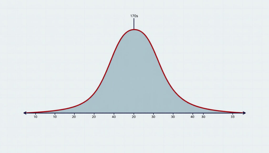
Standard deviation serves as a foundational building block in probability theory and inferential statistics. In a normal distribution, approximately 68% of data falls within one standard deviation of the mean, about 95% within two standard deviations, and roughly 99.7% within three standard deviations. This relationship, known as the empirical rule, allows analysts to make probabilistic statements about where values likely reside in a dataset.
Beyond normal distributions, standard deviation appears in hypothesis testing, confidence intervals, and quality control charts. Financial analysts use it to measure investment volatility, researchers employ it to assess experimental reliability, and manufacturers apply it to monitor production consistency. The measure’s versatility stems from its ability to translate complex datasets into a single interpretable value that facilitates comparison and decision-making.
Quick Reference Grid
Typical distance of data points from the mean
σ (population), s (sample)
Measuring spread and variability
Same as original data
Key Insights
- Standard deviation measures dispersion, not central tendency
- Low SD indicates predictable, tightly clustered data
- High SD signals greater variability and potential outliers
- Values cannot be negative, as they derive from squared deviations
- SD uses original units, making interpretation more intuitive than variance
- Comparing SDs only works meaningfully when datasets share similar means
Snapshot Facts
| Term | Symbol | Formula Snippet | Example Value |
|---|---|---|---|
| Population SD | σ | sqrt(Σ(x-μ)²/N) | 2.5 |
| Sample SD | s | sqrt(Σ(x-x̄)²/(n-1)) | 2.7 |
| Population Variance | σ² | Σ(x-μ)²/N | 6.25 |
| Sample Variance | s² | Σ(x-x̄)²/(n-1)) | 7.29 |
How to Calculate Standard Deviation: Step-by-Step Guide
Calculating standard deviation involves a systematic process that transforms raw data into a meaningful measure of spread. While software tools can perform these calculations automatically, understanding the step-by-step process clarifies what the final number represents and helps you catch potential errors in data entry or interpretation.
Formula Breakdown
Two distinct formulas exist depending on whether you analyze a complete population or a sample from a larger group. The population standard deviation formula divides by N (the total number of data points), while the sample standard deviation formula divides by n-1 (one less than the sample size). This difference might seem minor but significantly affects results, particularly for smaller datasets.
The population variance formula appears as σ² = Σ(xᵢ – μ)² / N, where μ represents the population mean and N counts all observations. Taking the square root of this variance yields the population standard deviation: σ = √σ². For samples, the formulas become s² = Σ(xᵢ – x̄)² / (n-1) and s = √s², where x̄ denotes the sample mean and n represents the sample size.
The division by n-1 instead of n in sample calculations serves a specific purpose: it corrects for the bias that occurs when estimating population spread from sample data. This correction, known as Bessel’s correction, ensures that the sample standard deviation better estimates the true population standard deviation.
Manual Calculation Example
Consider a dataset of test scores: 4, 5, 5, 5, 7, 8, 8, 8, 9, 10. With N = 10 data points, the mean equals 69/10 = 6.9. Calculating each deviation from the mean and squaring it yields: (4-6.9)² = 8.41, (5-6.9)² = 3.61, and so on through all ten values. The sum of squared deviations totals 36.9.
For the population calculation, variance equals 36.9 / 10 = 3.69, making the standard deviation √3.69 ≈ 1.92. If this same data represents a sample rather than a complete population, variance becomes 36.9 / 9 = 4.1, and the standard deviation increases to √4.1 ≈ 2.02. The sample SD proves slightly higher because dividing by the smaller denominator produces a larger result that better estimates the true population spread.
Another example with data: 2, 7, 3, 12, 9 demonstrates the process with five values. The mean calculates to 33/5 = 6.6. Squared deviations sum to approximately 69.44, giving a population variance of 13.89 and a standard deviation of approximately 3.73. This higher value reflects the greater spread in this dataset, where the minimum (2) and maximum (12) differ by 10 units compared to a 6-unit spread in the test scores example.
Using Spreadsheets and Calculators
Modern spreadsheet software includes built-in functions that automate standard deviation calculations. In Excel or Google Sheets, the STDEV.P function calculates population standard deviation while STDEV.S computes the sample version. These functions handle large datasets efficiently and reduce the risk of arithmetic errors that plague manual calculations.
Online calculators offer another convenient option, particularly for quick checks or learning purposes. Most allow you to input raw data values and select whether to treat the dataset as a population or sample. Some advanced tools display intermediate steps, helping you verify each stage of the calculation process.
Population vs. Sample Standard Deviation
Understanding when to use population versus sample formulas ranks among the most important practical decisions in statistical analysis. Using the wrong formula produces systematically biased results that could lead to incorrect conclusions in research, business decisions, or quality control applications.
Key Differences in Formulas
The fundamental distinction lies in the denominator. Population calculations divide by N (the count of all data points in the dataset), while sample calculations divide by n-1. This difference stems from how samples interact with the populations they represent. When calculating from a sample rather than the complete population, dividing by n-1 provides a better estimate of the true population standard deviation.
The symbol convention reinforces this distinction: σ (sigma) represents population standard deviation, while s represents sample standard deviation. In academic papers, technical reports, and professional contexts, these symbols carry specific meaning about the nature of the data and the analytical approach used.
When to Use Each
Use population standard deviation when you have data from every member of the group you are analyzing. This scenario commonly arises in quality control, where you examine every product from a specific production run, or in organizational studies where you analyze all employees in a department. Population calculations produce the exact spread for your defined dataset.
Use sample standard deviation whenever your data represents a subset drawn from a larger population that you wish to understand. Survey research exemplifies this scenario: researchers collect responses from a sample and use sample SD to estimate what the full population’s variability would look like. Medical studies, market research, and most experimental science rely on sample calculations for this reason.
Treating sample data with population formulas underestimates the true variability in the underlying population. This bias becomes more pronounced with smaller sample sizes, making formula selection especially critical for pilot studies or preliminary research with limited participants.
| Aspect | Population | Sample |
|---|---|---|
| Variance Divider | N (total items) | n-1 (sample size minus one) |
| SD Symbol | σ | s |
| Result Characteristic | Exact for the defined dataset | Slightly larger, better population estimate |
| Example Effect | Lower calculated value | Higher calculated value |
Interpreting Standard Deviation Values
A standard deviation value alone provides limited insight. Interpretation requires context, typically involving comparison to a mean, comparison to other datasets, or reference to known distribution properties. The same SD value might indicate very different situations depending on the scale and nature of the data being analyzed.
Low, Medium, High: What They Indicate
A low standard deviation relative to the mean suggests data points cluster closely around the center value. In manufacturing, this indicates consistent, reliable production. In investment portfolios, it suggests stable returns with limited volatility. In educational testing, it might reflect homogeneous student performance across a specific group.
A high standard deviation indicates substantial spread, with values potentially ranging widely from the mean. This could represent genuinely diverse populations, volatile markets, inconsistent processes, or measurement error. High SD values deserve investigation to determine whether they reflect true variability or data quality issues.
Direct comparison of SD values only produces meaningful conclusions when datasets share similar scales and means. An SD of 5 carries very different implications for test scores ranging from 0 to 100 versus for temperatures ranging from -40 to 50 degrees. Coefficient of variation (standard deviation divided by mean) provides a scale-independent alternative for comparing variability across different contexts.
Connection to Normal Distribution
In normally distributed data, standard deviation takes on special significance through the empirical rule. Approximately 68% of observations fall within one SD of the mean, roughly 95% within two SDs, and about 99.7% within three SDs. This pattern enables quick probabilistic reasoning about where values likely reside without performing complex calculations.
Consider exam scores with a mean of 75 and standard deviation of 10. The empirical rule suggests approximately 68% of students scored between 65 and 85. About 95% scored between 55 and 95, and nearly all (99.7%) fell between 45 and 105. This framework helps educators set grading boundaries and helps students understand score distributions relative to their own performance.
The empirical rule applies specifically to normal distributions. Data exhibiting skewness, bimodality, or other non-normal patterns may not follow these percentages. Always visualize your data distribution before applying rules based on normality assumptions.
Standard Deviation vs. Variance and Other Measures
Standard deviation exists within a family of spread measures, each with distinct properties and appropriate use cases. Understanding how SD relates to variance, range, and other metrics helps you select the right tool for any analytical situation and avoid common misinterpretations.
Variance Explained
Variance represents the average of squared deviations from the mean, calculated by summing all squared differences between each data point and the mean, then dividing by the appropriate count (N for populations, n-1 for samples). Variance and standard deviation express the same underlying concept of spread, but variance uses squared units rather than original data units.
The relationship is straightforward: standard deviation equals the square root of variance. If variance equals 9, standard deviation equals 3. If variance equals 25, standard deviation equals 5. This mathematical connection means that whichever measure you calculate, you can easily derive the other by taking or squaring the square root.
Practical interpretation favors standard deviation because it maintains the original measurement units. A dataset of heights measured in centimeters yields a variance expressed in square centimeters, which lacks intuitive meaning. The corresponding standard deviation in centimeters directly relates to the original measurements. Variance calculations remain important in theoretical statistics and certain advanced applications, but standard deviation provides more accessible interpretations for most practical purposes.
Standard Deviation vs. Standard Error
Standard error measures the precision of a sample statistic, typically the sample mean, rather than the spread within a dataset. While standard deviation describes variability within data, standard error describes how much a sample statistic would vary if you drew multiple samples from the same population. Standard error equals standard deviation divided by the square root of sample size.
As sample size increases, standard error decreases, reflecting greater precision in estimating population parameters. This relationship highlights an important distinction: collecting more data reduces estimation uncertainty (standard error) but does not change the underlying data variability (standard deviation). Larger samples provide better estimates of the true population mean but do not make the population itself more homogeneous.
How to Find Standard Deviation by Hand
The manual process follows a clear sequence: first calculate the mean, then find each deviation by subtracting the mean from every data point, square each deviation to eliminate negatives, sum all squared deviations, divide by the appropriate count to obtain variance, and finally take the square root to reach standard deviation. This six-step process applies to both population and sample calculations, with the division step determining which formula applies.
Working through an example with heights of adult dogs from a sample might involve values like 450mm, 600mm, 470mm, 520mm, and 550mm. The mean equals 2590/5 = 518mm. Deviations from this mean are -68, 82, -48, 2, and 32 millimeters. Squaring these gives 4624, 6724, 2304, 4, and 1024, which sum to 14680. Dividing by n-1 = 4 yields a sample variance of 3670, making the sample standard deviation approximately 60.6mm. Research examples may report slightly different values depending on specific datasets and rounding conventions.
Real-World Applications of Standard Deviation
Standard deviation appears across numerous fields, providing practical value beyond academic exercises. These applications demonstrate how the measure translates into actionable insights for decision-making, risk assessment, and quality improvement across diverse industries.
Applications in Finance and Investing
Investment analysts rely heavily on standard deviation to quantify price volatility and risk. A stock with high historical standard deviation in returns exhibits greater price swings, presenting both higher potential rewards and greater potential losses. Portfolio managers use SD to assess diversification benefits and optimize asset allocation strategies that balance expected return against variability in outcomes.
Fund performance reports typically display standard deviation alongside average returns, allowing investors to evaluate whether higher average returns justify increased volatility. Two funds with identical average returns may carry very different risk profiles if one shows consistently moderate results while the other swings between exceptional gains and significant losses.
Healthcare and Medicine
Medical researchers apply standard deviation when analyzing clinical measurements, treatment outcomes, and patient characteristics. Blood pressure readings, cholesterol levels, and recovery times all get characterized by central tendency and spread. Understanding this variability helps clinicians establish reference ranges, identify abnormal results, and evaluate treatment effectiveness across diverse patient populations.
Drug trials use standard deviation to assess response variability across participants. A new medication showing consistent results across patients (low SD) demonstrates more predictable effects than one with highly variable responses (high SD). This information guides both regulatory decisions and prescribing recommendations.
Manufacturing and Quality Control
Production facilities monitor standard deviation to ensure consistent product quality. Specifications define acceptable ranges for critical dimensions, and ongoing production samples get measured to verify that variability remains within acceptable limits. When SD increases beyond historical baselines, investigation into process changes, equipment issues, or material inconsistencies follows.
Statistical process control charts plot sample means alongside control limits derived from standard deviation. Points falling outside these limits trigger alerts for potential problems. This application demonstrates how standardized measures enable consistent quality monitoring across different products, facilities, and industries.
History and Development of Standard Deviation
The concept of measuring data dispersion evolved over centuries, with contributions from mathematicians seeking to characterize observation errors and natural variation. Understanding this historical context illuminates why standard deviation became the preferred measure and how statistical thinking developed alongside broader scientific advancement.
- Early 1800s: Carl Friedrich Gauss formalized the method of least squares and introduced concepts underlying modern dispersion measurement during his work on astronomical calculations and error analysis.
- 1823: Pierre-Simon Laplace refined approaches to measuring probability distributions and dispersion, building on Gauss’s foundational work.
- Late 1800s: Karl Pearson introduced the term “standard deviation” and established its notation, cementing the measure’s place in statistical vocabulary.
- Early 1900s: Ronald Fisher developed the mathematical framework connecting standard deviation to inferential statistics, hypothesis testing, and experimental design.
- Mid-1900s onward: Widespread adoption across scientific disciplines, business applications, and computational tools transformed standard deviation from an academic concept into a practical tool for decision-making.
What Standard Deviation Cannot Tell You
Standard deviation provides valuable information about spread, but several aspects of data distribution escape its characterization. Recognizing these limitations helps prevent overreliance on any single metric and encourages comprehensive data exploration.
Standard deviation is a precise mathematical measure when calculated correctly. However, uncertainty arises in how we apply it. When working with samples rather than complete populations, standard deviation becomes an estimate that carries its own uncertainty, typically expressed through confidence intervals rather than as a fixed value.
| What SD Reveals | What SD Hides |
|---|---|
| Overall spread around the mean | Direction of skewness |
| Typical distance from center | Presence of multiple modes |
| Consistency of measurements | Individual outlier values |
| Relative variability comparison | Range of extreme values |
Limitations and Alternatives
Standard deviation proves sensitive to extreme values because it squares every deviation before averaging. A single outlier can dramatically inflate SD even when all other values cluster tightly. In such cases, the interquartile range (IQR) provides a more robust alternative, measuring spread based on the middle 50% of data while ignoring both tails of the distribution.
Skewed distributions present another challenge, as standard deviation assumes symmetry around the mean. Highly skewed data may require transformation before analysis or alternative metrics that do not assume normality. Visualization through histograms and box plots remains essential for understanding data shape before relying on standard deviation as a summary measure.
Understanding Through Expert Perspectives
Statistical authorities emphasize standard deviation’s role as a fundamental measure of dispersion in quantitative analysis. The National Institute of Standards and Technology references standard deviation in its statistical handbook as a primary tool for characterizing measurement uncertainty and quality assurance protocols.
Standard deviation provides the foundation for understanding how data varies around its average value, enabling meaningful comparisons across different datasets and contexts.
Educational resources from institutions like Khan Academy and Statistics Canada stress the practical interpretation of standard deviation, focusing on how the measure translates abstract data into understandable patterns. Their materials emphasize that while calculation involves mathematical steps, the ultimate goal involves gaining intuitive insight into data behavior and variability.
When comparing datasets with similar means, the dataset with the lower standard deviation shows values clustered more tightly around the average, indicating greater consistency or predictability.
Putting Standard Deviation Into Practice
Standard deviation transforms raw numerical data into actionable insight by quantifying how values distribute around their average. Whether evaluating investment volatility, monitoring manufacturing quality, or interpreting medical research, this measure provides the foundation for understanding variability in ways that simple averages cannot capture.
The distinction between population and sample calculations deserves careful attention, as formula selection directly impacts results and interpretations. Population formulas apply to complete datasets, while sample formulas provide better estimates when working with subsets of larger populations. For most practical applications involving sampling, the corrected sample formula prevents systematic underestimation of true variability.
Combining standard deviation knowledge with visualization techniques, contextual understanding, and awareness of limitations equips you to make informed decisions based on data. The measure serves as a starting point rather than a complete solution, inviting deeper exploration of patterns, causes, and implications that numbers alone cannot reveal. Understanding conversion between different measurement systems, such as 8 Oz to Grams – Exact 226.8g Conversion Guide, demonstrates how standardization enables meaningful comparison across contexts, much as standard deviation enables comparison across different datasets.
Frequently Asked Questions
How is standard deviation used in real life?
Standard deviation applies in finance to measure investment volatility, in healthcare to assess measurement variability in vital signs and lab results, in manufacturing to monitor product quality consistency, and in sports to evaluate player performance consistency. Any situation requiring understanding of data spread benefits from SD analysis.
What is standard deviation vs mean?
The mean represents the average value in a dataset, while standard deviation measures how far typical values fall from that average. A dataset with a mean of 50 and SD of 5 shows most values clustering between 45 and 55, while the same mean with an SD of 15 indicates much wider variation from the center.
Can standard deviation be negative?
Standard deviation can never be negative because it is calculated by squaring deviations (eliminating negatives), summing them, dividing, and finally taking the square root. Since all intermediate values remain non-negative and the square root of any non-negative number is non-negative, SD is always zero or positive.
What does a low standard deviation mean?
A low SD indicates data points cluster closely around the mean, suggesting consistency, predictable behavior, or homogeneous populations. In quality control, low SD signals reliable production. In investments, it suggests stable returns. In measurements, it indicates high precision.
How do you interpret standard deviation results?
Interpret SD by considering the context, scale, and comparison to other measures. A SD of 10 has different meanings for exam scores (range 0-100) versus temperatures (range -50 to 50). Compare SD to the mean using coefficient of variation for scale-independent interpretation.
What is the difference between standard deviation and variance?
Variance equals the average of squared deviations from the mean, while standard deviation equals the square root of variance. Variance uses squared units (which lack intuitive meaning), while SD uses original data units. SD is the more practical and commonly reported measure.
Why is sample standard deviation higher than population standard deviation?
Sample SD divides by n-1 rather than n, which compensates for the bias that occurs when estimating population spread from sample data. This correction, called Bessel’s correction, produces a slightly higher value that better estimates the true population variability.
What is a good standard deviation value?
No universal “good” SD exists because interpretation depends entirely on context and scale. Compare SD to the mean using coefficient of variation, or compare SD values across similar datasets to identify relative consistency. Context-specific benchmarks from industry standards or historical data provide the most meaningful reference points.
More related posts
 Canada Income Tax Calculator: Top Tools for 2025-2026
 8 Oz to Grams – Exact 226.8g Conversion Guide
 Callum Turner: Actor, Net Worth, Relationship with Dua Lipa
 Average Height for Women in Canada: Stats & Global Comparison
 124 USD to CAD Today: Live Rates and Converter Comparison
 Whoopi Goldberg: Health Scare, Career, and Personal Life
 Nova Scotia School Closures – Current Status All Regions Open
 Selena Gomez: Lupus, Net Worth & Life in 2025